Edit (2016-05-31): Added a hypothesis for why my results differ somewhat from Erin Becker's. Briefly: I removed individuals who taught before they were officially certified.
A couple weeks ago, Greg Wilson asked the Software Carpentry community for feedback on a collection of data about the organization's instructors, when they were certified, and when they taught. Having dabbled in survival analysis, I was excited to explore the data within that context.
Survival analysis is focused on time-to-event data, for example time from birth until death, but also time to failure of engineered systems, or in this case, time from instructor certification to first teaching a workshop. The language is somewhat morbid, but helps with talking precisely about models that can easily be applied to a variety of data, only sometimes involving death or failure. The power of modern survival analysis is the ability to include results from subjects who have not yet experienced the event when data is collected. After all, studies rarely have the funding or patience to continue indefinitely. and excluding those data points entirely would falsely inflate rate estimates. Instead, the absence of an event for an individual during the study is useful information that contributes to the precise estimation of rates.
Let's grab the Software Carpentry data and take a look.
curl -O http://software-carpentry.org/files/2016/05/teaching-stats-2016-05.csv
Now in Python:
import pandas as pd
import numpy as np
import patsy
import statsmodels.api as sm
import matplotlib.pyplot as plt
import seaborn as sns

# If you're using jupyter:
%matplotlib inline

raw_data = pd.read_csv('teaching-stats-2016-05.csv').sort_values('Person')

print(raw_data.tail(10))
      Person   Certified      Taught
1781   11268  2016-03-16         NaN
1782   11278  2016-03-29         NaN
1783   11280  2016-04-19         NaN
1784   11292  2016-02-29         NaN
1785   11293  2016-03-01         NaN
1558   11294  2016-04-25  2016-04-18
1557   11294  2016-04-25  2016-02-02
1559   11295  2016-04-25  2016-02-02
1786   11298  2016-04-21         NaN
1787   11311  2016-04-19         NaN
This data is arranged as three columns: a ID number for each person,
the date they were certified, and the date they taught.
Individuals who have taught more than once have more than one row,
and individuals who have been certified but have not yet taught have one
row where taught is NaN.
In our analysis, each certified instructor will be a data point with a certification date, a date of first teaching, second teaching, etc. Let's rearrange our data to reflect this structure using pandas split-apply-combine functionality.
def get_person_details(data):
    data = data.copy().sort_values('Taught')
    certified = data.Certified.drop_duplicates()
    assert len(certified) == 1
    taught = data.Taught.drop_duplicates()

    if len(taught) < 2:
        taught_first = taught.iloc[0]
        taught_second = np.nan
    else:
        taught_first = taught.iloc[0]
        taught_second = taught.iloc[1]

    return pd.Series({'certified': certified.iloc[0],
                      'taught_first': taught_first,
                      'taught_second': taught_second,
                      'taught_count': taught.notnull().sum()})

data = raw_data.groupby('Person').apply(get_person_details)

print(data.head())
         certified  taught_count taught_first taught_second
Person
48      2014-05-04             1   2014-09-11           NaN
75      2013-07-20            15   2013-03-20    2013-03-24
85      2014-12-23             4   2015-03-06    2015-06-17
87      2013-11-25             4   2014-05-12    2015-03-20
135     2015-02-03             1   2015-09-03           NaN
And some calculations
data.certified = pd.to_datetime(data.certified)
data.taught_first = pd.to_datetime(data.taught_first)
data.taught_second = pd.to_datetime(data.taught_second)
data['has_taught'] = data.taught_count > 0
data['has_taught_multiple'] = data.taught_count > 1
data['time_to_taught_first'] = (data.taught_first -
                                data.certified).dt.days
data['time_to_taught_second'] = (data.taught_second -
                                 data.certified).dt.days
data['time_between_first_second'] = (data.time_to_taught_second -
                                     data.time_to_taught_first)
data['year_certified'] = data.certified.dt.year
I'd like to include data on how long instructors have been certified, since, for instructors who have not taught, thats how long they have gone without teaching. To get this value I need to a collection date for the data, which I don't know. For now, I'll use June 1st since I know the data was from May.
COLLECTION_DATE = pd.datetime(year=2016, month=6, day=1)
data['time_since_certified'] = (COLLECTION_DATE - data.certified).dt.days
data['time_since_taught_first'] = (COLLECTION_DATE - data.taught_first).dt.days
I'll take a quick peek at the key column.
print(data[['time_to_taught_first']].head())
        time_to_taught_first
Person
48                     130.0
75                    -122.0
85                      73.0
87                     168.0
135                    212.0
Some people (Person 75, for instance) taught their first workshop before they were officially certified. I don't have any idea how to include them in the analysis, so I will be removing them from this point forward. I believe that the removal of these individuals explain differences between my results and the analysis posted to the Software Carpentry blog by Erin Becker.
data = data[(data.time_to_taught_first > 0) |
            data.time_to_taught_first.isnull()]
Visualization is usually a good idea:
data.time_to_taught_first.plot.hist(bins=data.taught_count.max())
plt.xlabel('Days between certification and first teaching')
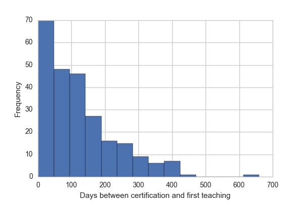
print("{} of {} instructors have not yet taught."
          .format(sum(~data.has_taught), len(data)))
Of the 474 instructors in this data, 228 have not yet taught.
Now we jump into the survival analysis. I'm going to compare time-to-first-teaching to the year in which instructors were certified. This is mostly because I want a covariate here, and I don't have access to more interesting ones, e.g. what style of training it was (online, 2-day, etc.).
# We'll be modifying our data, so a copy will keep the original pristine.
_data = data.copy()

# If individuals have not yet taught as of data collection,
# then we will censor them.
# statsmodels requires this time-to-censoring be in the same column as the
# time-to-event.
_data.time_to_taught_first.fillna(_data.time_since_certified, inplace=True)

# Fit a proportional hazards model, comparing certification year.
# "Sum" stands for sum-to-zero coding for the design matrix.
ydm, xdm = \
    patsy.dmatrices('time_to_taught_first ~ C(year_certified, Sum)',
                    data=_data, return_type='dataframe')
# Remove the intercept term.
xdm = xdm.drop('Intercept', axis='columns')

# Right censor for individuals who have not yet taught by the date
# of this data collection.
fit1 = sm.PHReg(ydm, xdm, status=_data.has_taught).fit()
The most widely used model in survival analysis is called the proportional hazards model. In the process of testing the significance of our covariates in this model, a survival curve is calculated. In this case, because of the coding for certification year in the design matrix, this "baseline" curve represents the mean of annual means.
sf = fit1.baseline_cumulative_hazard[0]
plt.plot(sf[0], sf[2])
plt.ylim(0, 1)
plt.xlabel("Days post-certification")
plt.ylabel("Fraction instructors not taught")
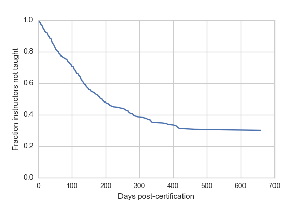
The key figure in survival analysis is the survival curve, or its derivative the hazard function. Survival curves plot the number or percentage of individuals who have not yet experienced the event after a given amount of time. In the case of this data, the survival curve reflects the fraction of instructors who have not yet taught by a given number of days after they were certified.
Despite the fact that about 50% of certified instructors have not yet taught, many of these are recently trained and we expect them to teach in the future. 50% of certified instructors teach by 200 days. After more than a year, however, the survival curve flattens out. Approximately 30% of instructors get to 400 days without having taught and at 600 days about the same fraction have still not taught. If we want to extrapolate beyond the data (always a bad idea) then we might predict that these instructors will never teach.
We can also test the effect of certification year on time to first workshop.
print(fit1.summary())
                                   Results: PHReg
====================================================================================
Model:                       PH Reg                        Sample size:          474
Dependent variable:          time_to_taught_first          Num. events:          246
Ties:                        Breslow
------------------------------------------------------------------------------------
                                log HR log HR SE   HR      t    P>|t|  [0.025 0.975]
------------------------------------------------------------------------------------
C(year_certified, Sum)[S.2012]  0.1382    0.5705 1.1482  0.2422 0.8086 0.3753 3.5124
C(year_certified, Sum)[S.2013]  0.2230    0.2268 1.2498  0.9830 0.3256 0.8012 1.9493
C(year_certified, Sum)[S.2014] -0.1383    0.1789 0.8708 -0.7732 0.4394 0.6132 1.2366
C(year_certified, Sum)[S.2015]  0.0205    0.1730 1.0207  0.1183 0.9058 0.7272 1.4327
====================================================================================
Confidence intervals are for the hazard ratios
We see no significant deviation from the average year for any of the 4 years of certification data.
Just for fun, let's go even further with this data. Of the 246 instructors who have taught at least once, 131 have taught a second time. Can we predict the time after first teaching that it takes to teach again?
_data = data.copy()
_data = _data[_data.time_to_taught_first.notnull()]

# Fill in dates for right censoring.
_data.time_between_first_second.fillna(_data.time_since_taught_first, inplace=True)

# Fit a proportional hazards model using time between certification and first taught.
ydm, xdm = patsy.dmatrices('time_between_first_second ~ time_to_taught_first',
                           data=_data, return_type='dataframe')
xdm = xdm.drop('Intercept', axis='columns')  # Remove the intercept term

# Right censor for individuals who have not yet taught a second time.
fit2 = sm.PHReg(ydm, xdm, status=_data.has_taught_multiple).fit()

# The baseline hazard is the probability of having not taught a second
# time by a given day for someone who taught at day 0 of being certified.
sf = fit2.baseline_cumulative_hazard[0]
plt.plot(sf[0], sf[2])
plt.ylim(0, 1)
plt.xlabel("Days post-first-teaching")
plt.ylabel("Fraction instructors not taught second time")
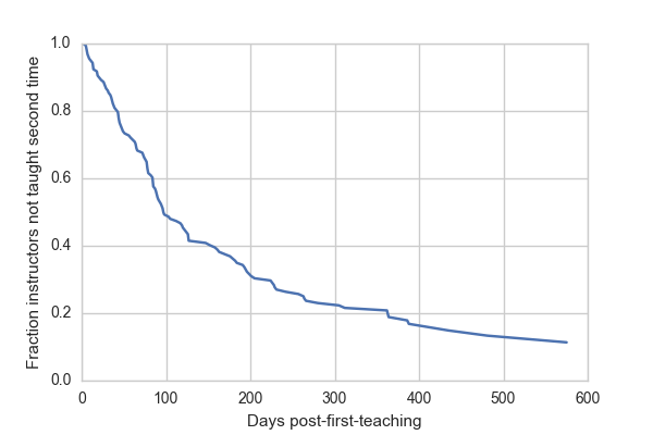
The baseline survival curve reflects expectations for a theoretical individual who taught immediately upon being certified (day 0). For these folks, we expect 50% to teach again within 100 days, and almost 80% within a year.
Let's take a look at the effect of time-to-first-teaching on time to teaching again.
print(fit2.summary())
                              Results: PHReg
==========================================================================
Model:                  PH Reg                        Sample size:     246
Dependent variable:     time_between_first_second     Num. events:     131
Ties:                   Breslow
--------------------------------------------------------------------------
                      log HR log HR SE   HR      t    P>|t|  [0.025 0.975]
--------------------------------------------------------------------------
time_to_taught_first -0.0045    0.0010 0.9955 -4.3474 0.0000 0.9935 0.9975
==========================================================================
Confidence intervals are for the hazard ratios
We find a highly significant effect of time-to-first-teaching.
The hazard ratio estimate is 0.9955. We can interpret this to mean that the per-day probability of teaching again goes down by 0.45% for every day between certification and teaching the first time. This isn't all that surprising; individuals who are able to teach soon after being certified are probably both enthusiastic and have more time to devote to teaching.
That's all I've got. Thanks for reading. I'd love to hear what you think and if you spot any glaring mistakes in my analysis. All of the code to do this is available on github. If you have ideas for additional analysis please leave a comment here, submit an issue to the github repository, or even better, a pull-request.
Comments